Microsoft Excel is one of the most powerful spreadsheet tools, with an impressive collection of built-in tools and features. In this article, you'll learn how powerful Excel formulas and conditional formatting can be, with three helpful examples.
We've covered several different ways to make better use of Excel, such as using it to create your own calendar template or using it as a project management tool.
Much of the power lies behind the Excel formulas and rules that you can write to manipulate data and information automatically, no matter what data you insert into the spreadsheet.
Let's dive into how you can use formulas and other tools to make better use of Microsoft Excel.
One of the tools that people don't use often is conditional formatting. If you're looking for more advanced information on conditional formatting in Microsoft Excel, be sure to check out Sandy's article on formatting data in Microsoft Excel with conditional formatting.
With the use of Excel formulas, rules, or just a few really simple settings, you can transform a spreadsheet into an automated dashboard.
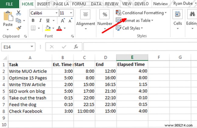
To access conditional formatting, simply click on Home and click the Conditional formatting toolbar icon.
Under Conditional Formatting, there are many options. Most of these are beyond the scope of this particular article, but most deal with highlighting, coloring, or shading cells based on the data within that cell.
This is probably the most common use of conditional formatting elements, such as turning a cell red with less than or greater than formulas. Learn more about how to use IF statements in Excel.
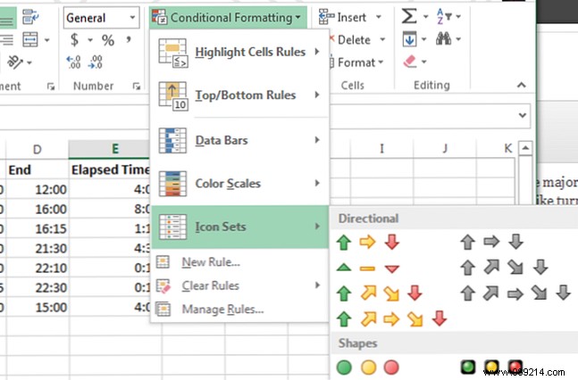
One of the least used conditional formatting tools is the Icon Sets option, which offers a large set of icons that you can use to turn an Excel data cell into a dashboard display icon.
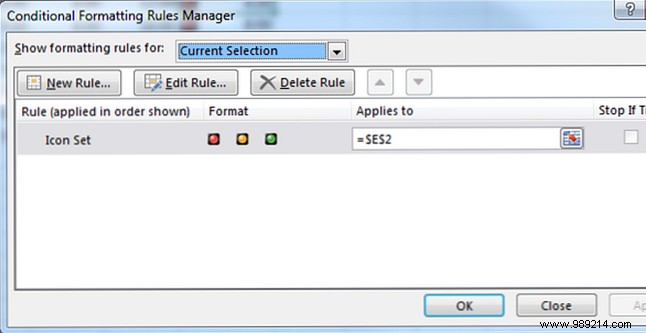
When you click Manage Rules , it will take you to the Conditional Formatting Rules Manager .
Depending on the data you selected before choosing the icon set, you will see the indicated cell in the Manager window, with the icon set you just chose.
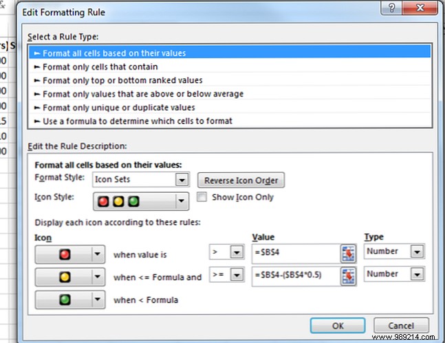
When you click Edit Rule , You will see the dialog where the magic happens..
This is where you can create the logic formula and equations that will display the dashboard icon you want.
This example dashboard will show the time spent on different tasks compared to the budgeted time. If you exceed half of the budget, a yellow light will appear. If you are completely over budget, it will turn red.
As you can see, this panel shows that the time budget is not successful.
Almost half of the time is spent over the budgeted amounts.
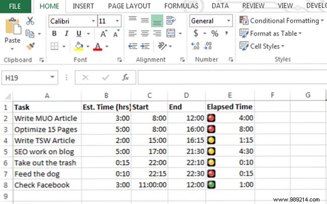
Time to refocus and better manage your time!
If you want to use more advanced features of Microsoft Excel, here is another one for you.
You're probably familiar with the VLookup function, which allows you to look in a list for a particular item in a column and return data from a different column in the same row as that item.
Unfortunately, the function requires that the item you're looking for in the list is in the left column, and the data you're looking for is on the right, but what if they are changed?
In the example below, what if I want to find the Task I did on 6/25/2018 from the following data?
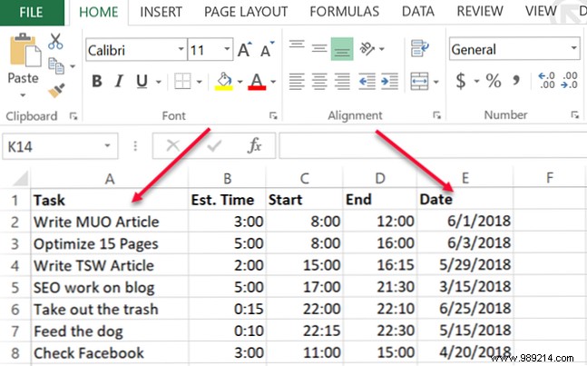
In this case, you're looking for values on the right and want to return the corresponding value on the left, as opposed to the way VLookup normally works.
If you read the professional Microsoft Excel user forums, you will find many people saying that this is not possible with VLookup, and that you have to use a combination of index and match functions to do this. That's not entirely true..
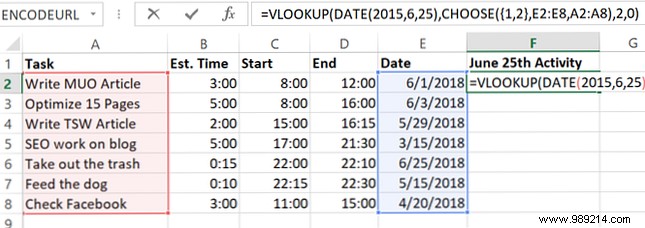
You can make VLookup work this way by nesting a CHOOSE function in it. In this case, the Excel formula would look like this:
"= VLOOKUP (FECHA (2018,6,25), ELEGIR (1,2, E2: E8, A2: A8), 2,0)"What this function means is that you want to look for the date 6/25/2013 in the lookup list and then return the corresponding value from the column index.
In this case, you'll notice that the column index is "2", but as you can see, the column in the table above is actually 1, to the right?
That's true, but what you're doing with the "CHOOSE" function is manipulating the two fields.
You are assigning reference “index” numbers to data ranges - assigning dates to index number 1 and tasks to index number 2.
So when you write "2" in the VLookup function, you actually mean index number 2 in the CHOOSE function. Cool right?
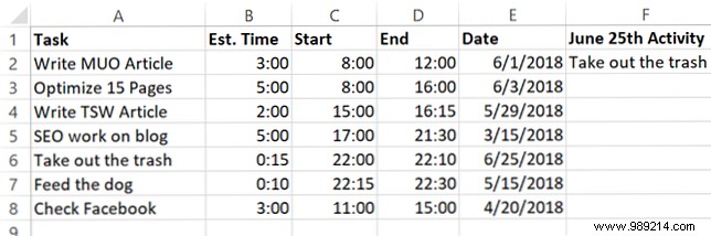
So now the VLookup uses the Date column and returns the data of the Task column, even though the task is on the left.
Now that you know this little detail, imagine what else you can do!
If you're trying to do other advanced data finding tasks, be sure to check out Dann's full article on finding data in Excel using the find functions.
Here is one more crazy Excel formula for you.
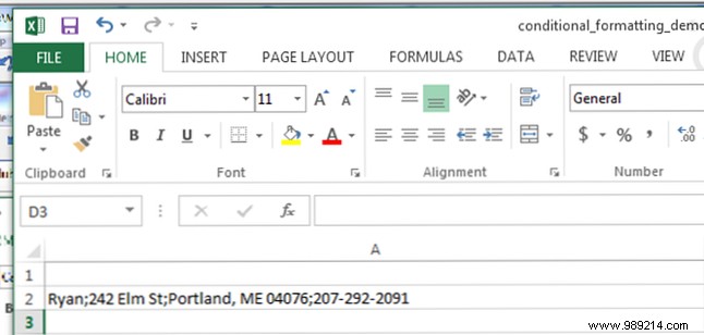
There may be cases where you import data into Microsoft Excel from an external source that consists of a delimited data string.
Once you input the data, you want to break down that data into the individual components. Here is an example of name, address, and phone number information delimited by the “;” character.
Here's how you can parse this information using an Excel formula (see if you can keep up with this madness in your head):
For the first field, to extract the leftmost element (the person's name), you simply use a LEFT function in the formula.
"= IZQUIERDA (A2, FIND ("; ", A2,1) -1)"This is how this logic works:
In this case, the leftmost text is “Ryan”. Mission accomplished.
But what about the other sections?
There may be easier ways to do this, but since we want to try to create the craziest Nested Excel formula possible (that actually works), we'll use a unique approach.
To extract the right parts, you need to nest multiple RIGHT functions to grab the section of text until the first one appears. “;” and run the LEFT function again. This is what it looks like to extract the street number part of the address.
"= IZQUIERDA ((DERECHA (A2, LEN (A2) -FIND ("; ", A2))), FIND ("; ", (DERECHA (A2, LEN (A2) -FIND ("; ", A2)) ), 1) -1) "It sounds crazy, but it is not difficult to reconstruct it. All I did is take this function:
DERECHA (A2, LEN (A2) -FIND (";", A2))And inserts it at every place in the LEFT function above where there is an "A2".
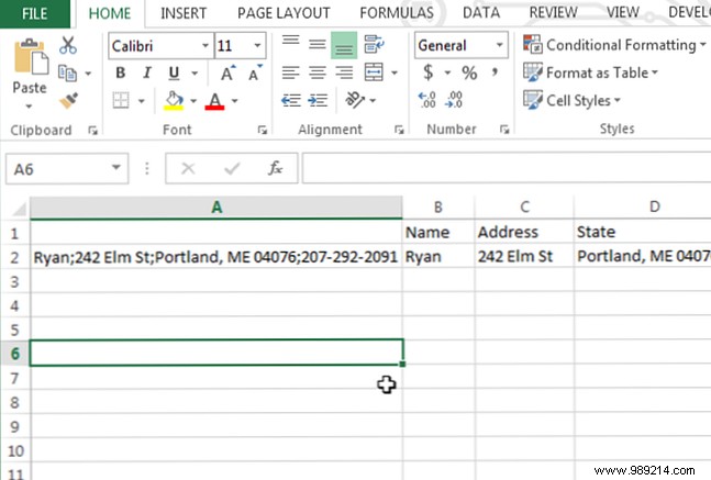
This correctly extracts the second section of the string.
Each subsequent section of the chain needs another nest created. So now you just take the crazy “RIGHT” equation you created for the last section, and then pass it into a new RIGHT formula with the previous RIGHT formula pasted into itself wherever you see it. “A2”. This is what it looks like.
(DERECHA ((DERECHA (A2, LEN (A2) -FIND (";", A2))), LEN ((DERECHA (A2, LEN (A2) -FIND (";", A2)))) - FIND ( ";", (DERECHA (A2, LEN (A2) -FIND (";", A2))))))Then take that formula and put it in the original LEFT formula where there is an "A2".
The final mind formula looks like this:
"= IZQUIERDA ((DERECHA ((DERECHA (A2, LEN (A2) -FIND ("; "))), LEN ((DERECHA (A2, LEN (A2) -FIND ("; ", A2))) ) -FIND (";", (RIGHT (A2, LEN (A2) -FIND (";" A2)))))) FIND (";", (RIGHT ((RIGHT (A2, LEN (A2) -FIND (";", A2))), LEN ((DERECHA (A2, LEN (A2) -FIND (";", A2)))) - FIND (";", (DERECHA (A2, LEN (A2) ) -FIND (";", A2))))))), 1) -1) "That formula correctly extracts "Portland, ME 04076" out of the original string.
To extract the next section, repeat the above process again.
Your Excel formulas can get really crazy, but all you're doing is cutting and pasting long formulas into themselves, make long nests that actually work.
Yes, this meets the "crazy" requirement. But let's be honest, there is a much easier way to achieve the same thing with a function.
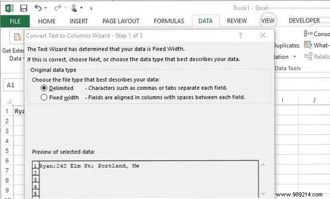
Just select the column with the delimited data, and then under Data menu item, select Text to Columns .
This will open a window where you can split the string by any delimiter you like.
In a couple of clicks, you can do the same thing as the crazy formula above... but where's the fun?
So there you have it. The above formulas demonstrate how much hype a person can get when creating Microsoft Excel formulas to accomplish certain tasks.
Sometimes those Excel formulas aren't really the easiest (or best) way to accomplish things. Most programmers will tell you to keep it simple, and that's as true with Excel formulas as it is with anything else.
If you really want to get serious about using Excel, you'll want to read our beginner's guide to using Microsoft Excel The Beginner's Guide to Microsoft Excel The Beginner's Guide to Microsoft Excel Use this beginner's guide to start your experience with Microsoft Excel. The basic spreadsheet tips here will help you start learning Excel on your own. Read more . Tiene todo lo que necesita para comenzar a aumentar su productividad con Excel..