Many people struggle with extracting information from complex cells in Microsoft Excel. The number of comments and questions in response to my article on How to extract a number or text from Excel with this function How to extract a number or text from Excel with this function How to extract a number or text from Excel with this function Mix numbers and Text in an Excel spreadsheet can present challenges. We'll show you how to change the format of your cells and numbers separate from the text. Read More Apparently it's not always clear how to isolate the desired data from an Excel sheet.
We've chosen some of the questions from that article to look at here, so you can see how the solutions work. Learning Excel Quickly 8 Tips to Learn Excel Quickly 8 Tips to Learn Excel Quickly Not as comfortable with Excel as you'd like? Get started with simple tips for adding formulas and managing data. Follow this guide and you'll be up to speed in no time. Read More
Reader Adrie asked the following question:
The fact that the numbers to extract have different lengths makes this a bit more complicated than just using the MID function, but by combining a few different functions, we can remove the left letters and the left letters. “X” and the numbers to the right, leaving only the desired numbers in a new cell.
Here is the formula we will use to solve this problem:
= VALOR (IZQUIERDA ((DERECHA (A1, (LEN (A1) -4))), ENCONTRAR ("X", A1) -5))
Let's start in the middle and work to see how it works. First, we'll start with the FIND function. In this case, we are using FIND("X",A1). This function searches through the text in cell A1 for the letter X. When it finds an X, it returns the position it is at. For the first entry, COIL112X2.5, for example, returns 8. For the second entry, it returns 7.
Next, let's look at the LEN function. This simply returns the length of the string in the cell minus 4. Combining that with the RIGHT function, we get the string in the cell minus the first four characters, which removes "COIL" from the beginning of each cell. The formula for this part looks like this:RIGHT(A1, (LEN(A1)-4)).
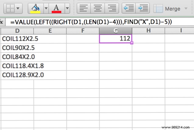
The next level is the LEFT function. Now that we have determined the position of the X with the FIND function and got rid of “COIL” with the RIGHT function, the LEFT function returns what is left. Let's break this down a bit more. This is what happens when we simplify those two arguments:
= IZQUIERDA ("112X2.5", (8-5)) The LEFT function returns the leftmost three characters of the string (the "-5" at the end of the argument ensures that the correct number of characters is removed when counting the first four characters of the string).
Finally, the VALUE function ensures that the returned number is formatted as a number, rather than as text. This example isn't as much fun as building a working game of Tetris in Excel 7 Fun and Weird Things You Can Create with Microsoft Excel 7 Fun and Weird Things You Can Create with Microsoft Excel Imagine Excel was fun! Excel offers ample scope for projects that go beyond its intended use. The only limit is your imagination. These are the most creative examples of how people use Excel. Read More
Reader Yadhu Nandan asked a similar question:
Another reader, Tim K SW, provided the perfect solution for this particular problem:
The formulas are quite simple, but if you are not familiar with the MID function, you may not understand how it works. MID takes three arguments:a cell, the number of characters where the result begins, and the number of characters to extract. MID(A1,10,4), for example, tells Excel to take four characters starting at the tenth character in the string.
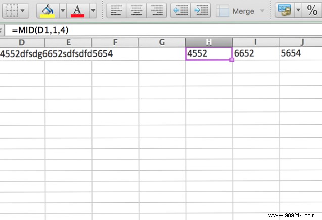
Using the three different MID functions in three cells pulls the numbers out of this long string of numbers and letters. Obviously, this method only works if you always have the same number of characters, both letters and numbers, in each cell. If the number of each varies, you'll need a much more complicated formula.
One of the most difficult requests posted in the article was this one, from reader Daryl:
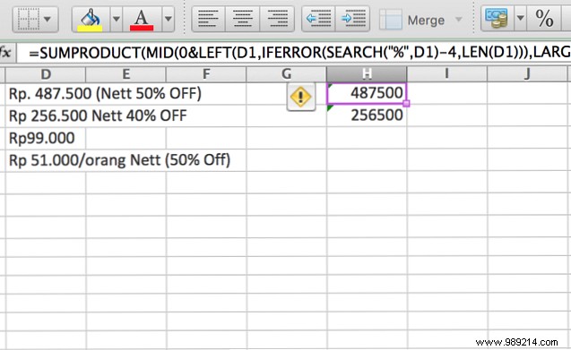
I spent some time working on this and couldn't find a solution so I went to Reddit. User UnretiredGymnast provided this long and very complex formula:
= SUMPRODUCTO (MEDIO (0 Y IZQUIERDA (A1, IFERROR (BÚSQUEDA ("%", A1) -4, LEN (A1))), GRANDE (ÍNDICE (NÚMERO (- IZQUIERDO (IZQUIERDA (A1, IFERROR (BÚSQUEDA ("%" , A1) -4, LEN (A1)), ROW ($ 1: $ 99), 1)) * ROW ($ 1: $ 99), 0), ROW ($ 1: $ 99)) + 1,1) * 10 ^ ROW ($ 1: $ 99) / 10) As you can see, decoding this formula is quite time consuming and requires a pretty solid understanding of many Excel functions. 16 Excel formulas to help you solve real life problems. 16 Excel formulas to help you solve real life problems. The right tool is half the job. Excel can solve calculations and process data faster than your calculator can. We show you the key Excel formulas and show you how to use them. Read more . To help figure out exactly what's going on here, we'll have to look at some features you may not be familiar with. The first is IFERROR, which catches an error (usually represented by a number sign, like #N/A or #DIV/0) and replaces it with something else. In the above, you will see IFERROR(SEARCH("%",A1)-4, LEN(A1)). Let's break this down.
IFERROR looks at the first argument, which is SEARCH("%",A1) -4. So if "%" appears in cell A1, its location is returned and four is subtracted. Yes “%” no appears in the string, Excel will create an error and the length of A1 is returned instead.
The other features you might not be familiar with are a bit simpler; SUMPRODUCT, for example, multiplies and then adds elements of arrays. LARGE returns the largest number in a range. ROW, combined with a dollar sign, returns an absolute reference to a row.
Seeing how all these functions work together isn't easy, but if you start in the middle of the formula and work your way out, you'll start to see what you're doing. It will take a while, but if you're interested in seeing exactly how it works, I recommend putting it in an Excel sheet and playing around with it. That's the best way to get an idea of what you're working with.
(Also, the best way to avoid a problem like this is to import your data in a clearer way. How to import data into your Excel spreadsheet in a clear and easy way. How to import data into your Excel spreadsheet in a clear way and easy. Import or export data to a spreadsheet? This tutorial will help you master the art of moving data between Microsoft Excel, CSV, HTML, and other file formats. Read More:It's not always an option, but it should be your first choice when it is.)
As you can see, the best way to solve any Excel problem is one step at a time:start with what you know, see what you get, and go from there. Sometimes you will end up with an elegant solution and sometimes you will end up with something that is really long, messy and complex. But as long as it works, you've succeeded!
And don't forget to ask for help. Do you need to learn Excel? 10 experts will teach you for free! Do you need to learn Excel? 10 experts will teach you for free! Learning to use the more advanced features of Excel can be difficult. To make it a little easier, we've tracked down the best Excel gurus that can help you master Microsoft Excel. Read more . There are some extremely talented Excel users out there and their help can be invaluable in solving a difficult problem.
Do you have any suggestions for solving difficult extraction problems? Do you know of any other solutions to the problems we addressed above? Share them and any feedback you have in the comments below!