Most of the time, finding a cell in an Excel spreadsheet is pretty easy; If you can't just scan the rows and columns for it, you can use CTRL + F to search for it. But if you are working with a huge spreadsheet How to Split a Huge Excel CSV Spreadsheet into Separate Files How to Split a Huge Excel CSV Spreadsheet into Separate Files One of the shortcomings of Microsoft Excel is the limited size of a sheet calculation. If you need to make your Excel file smaller or split a large CSV file, read on! Read More No matter the size of your Microsoft Excel document, they will be much more efficient.
This function allows you to specify a column and a value, and will return a value from the corresponding row of a different column (if that doesn't make sense, it will become clear in a moment). Two examples where you can do this are looking up an employee's last name by their employee number, or finding a phone number by specifying a last name. Here is the function syntax:
= VLOOKUP ([lookup_value], [table_array], [col_index_num], [range_lookup])
The [lookup_value] is the information you already have; for example, if you need to know what state a city is in, it would be the name of the city. [table_array] allows you to specify the cells in which the function will search for the lookup and return values. When selecting your range, make sure that the first column included in your array is the one that will contain your lookup value. This is critical. [col_index_num] is the number of the column that contains the return value.
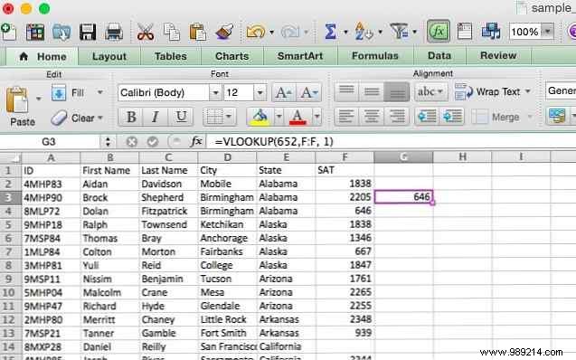
[range_lookup] is an optional argument, and takes 1 or 0. If you enter 1 or omit this argument, the function looks for the value you entered or the next lower number. So, in the image below, a VLOOKUP looking for an SAT score of 652 will return 646, since it is the closest number in the list that is less than 652, and [range_lookup] defaults to 1.
Let's take a look at how we could use this. As I have in my articles on Boolean operators in Microsoft Excel Mini Excel Tutorial:Using Boolean Logic to Process Complex Data Mini Excel Tutorial:Using Boolean Logic to Process Complex Data The logical operators IF, NOT, AND, and OR can help you get Excel novice to advanced user. We explain the basics of each feature and demonstrate how you can use them to get the best results. Read More and Advanced Counting and Adding Mini Excel Tutorial:Using Advanced Counting and Adding Functions in Excel Mini Excel Tutorial:Using Advanced Counting and Adding Functions in Excel Counting and adding formulas can seem mundane compared to more advanced Excel formulas. But they can help you save a lot of time when you need to gather information about the data in your spreadsheet. Read More It contains identification numbers, first and last names, city, state, and SAT scores. Let's say I want to find the SAT score of a person with the last name "Winters." VLOOKUP makes it easy. Here is the formula we would use:
= VLOOKUP ("Inviernos", C2: F101, 4, 0) Since SAT scores are the fourth column of the last name column, I've used 4 for the column index argument. Note that when searching for text, setting [range_lookup] to 0 is a good idea; Without it, you can get poor results. This is what Microsoft Excel gives us:
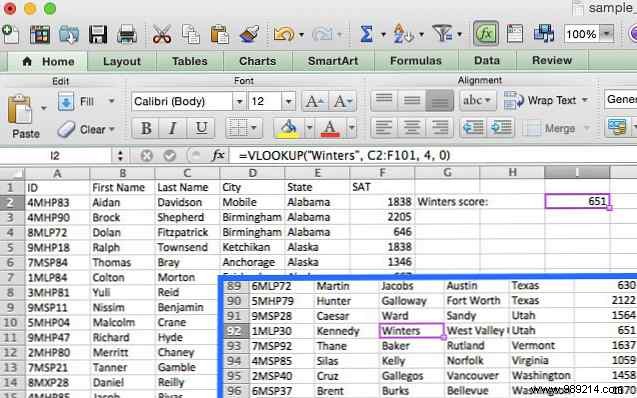
It returned 651, the SAT score belonging to the student named Kennedy Winters, who is in row 92 (shown in the box above). He would have taken much longer to scroll looking for the name than to quickly type the syntax!
VLOOKUP can also be very useful if you are using Microsoft Excel to do your taxes. Doing your taxes? 5 Excel formulas you should know doing your taxes? 5 Excel Formulas You Need to Know It's two days before your taxes are due and you don't want to pay another late filing fee. This is the time to harness the power of Excel to put everything in order. Read more.
Some things are good to remember when you are using VLOOKUP. First, as I mentioned above, make sure the first column in your range is the one that includes your lookup value. If it is not in the first column, the function will return incorrect results. If your columns are well organized, this shouldn't be a problem.
The second thing to note is that VLOOKUP will only return one value. If we had used "Georgia" as the lookup value, it would have returned the score of the first student from Georgia and given no indication that there are two students from Georgia.
Where VLOOKUP finds the corresponding values in another column, HLOOKUP finds the corresponding values in a different row. Since it's usually easier to scan the column headers until you find the right one and use a filter to find what you're looking for, HLOOKUP is best used when you have Really Large spreadsheets or you are working with values that are organized by time. Here is the syntax:
= HLOOKUP ([lookup_value], [table_array], [row_index_num], [range_lookup])
[lookup_value], again, is the value that you know and want to find a corresponding value for. [table_array] is the cells you want to search. [row_index_num] specifies the row where the return value will come from. And [range_lookup] is the same as above; leave blank to get the closest value when possible, or enter 0 to search for exact matches only.
For this example, I have created a new spreadsheet with generatorata.com. It contains a row for each state, along with an SAT score (we'll call it the average score for the state) for the years 2000-2014. We'll use HLOOKUP to find the average score in Minnesota in 2013. Here's how we'll do it:
= HLOOKUP (2013, A1: P51, 24)
(Note that 2013 is not in quotes because it is a number and not a string; also, the 24 comes from Minnesota in row 24.) As you can see in the image below, the score is returned:
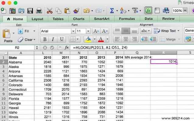
Minnesotans averaged a score of 1014 in 2013.
As with VLOOKUP, the lookup value must be in the first row of your table's array; this is rarely a problem with HLOOKUP, since it will usually use a column title for a lookup value. HLOOKUP also returns a single value.
INDEX and MATCH are two different functions, but when used together they can make searching a large spreadsheet much faster. Both features have drawbacks, but by combining them we will develop the strengths of both. First though, the syntax:
= INDICE ([array], [row_number], [column_number]) = MATCH ([lookup_value], [lookup_array], [match_type])
In INDEX, [array] is the array you will search. [row_number] and [column_number] can be used to limit your search; We'll take a look at that in a moment.
MATCH [lookup_value] is a search term that can be a string or a number; [lookup_array] is the array that Microsoft Excel will look up for the search term. [match_type] is an optional argument that can be 1, 0, or -1; 1 will return the largest value that is less than or equal to your search term; 0 will only return your exact term; and -1 will return the smallest value that is greater than or equal to your search term.
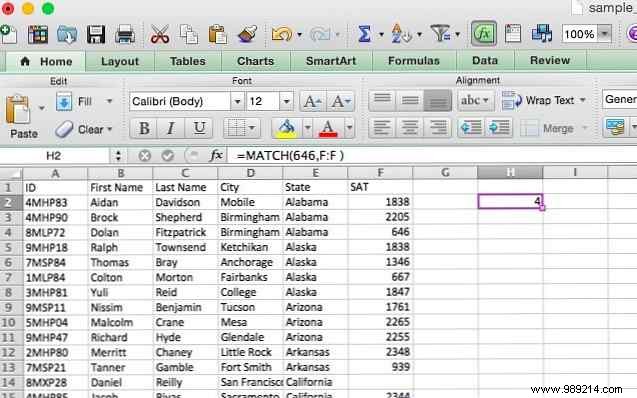
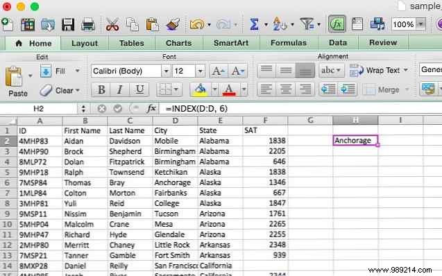
It may not be clear how we're going to use these two functions together, so I'll cover them here. MATCH takes a search term and returns a cell reference. In the image below, you can see that on a lookup for the value 646 in column F, MATCH returns 4.
INDEX, on the other hand, does the opposite:it takes a cell reference and returns the value in it. You can see here that when told to return the sixth cell in the City column, INDEX returns “Anchor,” the value from row 6.
What we're going to do is combine the two so that MATCH returns a cell reference and INDEX uses that reference to look up the value in a cell. Let's say you remember there was a student whose last name was Waters, and you want to see what this student's score was. Here is the formula we will use:
= ÍNDICE (F: F, PARTIDO ("Aguas", C: C, 0)) You'll notice that the match type is set to 0 here; when you're looking for a rope, that's what you'll want to use. This is what we get when we run that function:
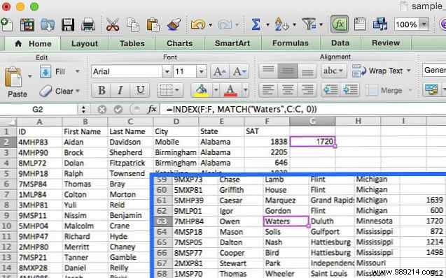
As you can see in the box, Owen Waters got 1720, the number that appears when we run the function. This may not seem all that useful when you can only look at a few columns, but imagine how much time you'd save if you had to do it 50 times on a large database spreadsheet Excel Vs Access:Can a Spreadsheet Replace a Database? data? Excel Vs. Access:Can a Spreadsheet Replace a Database? Which tool should I use to manage the data? Access and Excel both have data filtering, compiling, and querying. We will show you which one is the most suitable for your needs. Read More
Microsoft Excel has a host of extremely powerful features. 3 Crazy Excel Formulas That Do Amazing Things. 3 Crazy Excel Formulas That Do Amazing Things. Las fórmulas de formato condicional en Microsoft Excel pueden hacer cosas maravillosas. Aquí hay algunos trucos de productividad de fórmulas de Excel. Lea más, y los cuatro enumerados arriba simplemente rasguñan la superficie. Sin embargo, incluso con esta descripción general, debería poder ahorrar mucho tiempo cuando trabaja con hojas de cálculo grandes. Si desea ver cuánto más puede hacer con INDEX, eche un vistazo “El índice de imposición” en Microsoft Excel Hero.
¿Cómo ejecutar búsquedas en grandes hojas de cálculo? ¿Cómo has encontrado que estas funciones de búsqueda sean útiles?? Comparte tus pensamientos y experiencias a continuación!