Google Sheets is a popular Microsoft Excel alternative. As with other Google tools, Sheets is a core part of Google Drive. In this article, we've taken the liberty of diving deep and unearthing a handful of super-useful Google Sheets tricks that you may never have heard of before.
These Google Spreadsheet tricks are simple enough to learn and remember.
We have all encountered situations where we need third party calculators for exchange conversions. While there is nothing wrong with doing this, it is a tedious way of doing things. Google Sheets offers built-in currency conversion features that will help you convert from one currency to another in no time. Let's see how to use this feature.
Use the following syntax:
=* GOOGLEFINANCE ("MONEDA:") Let's break it down. The “from the currency symbol ” is the base currency you want to convert. The “to the currency symbol ” is the currency you want to convert the initial value to.
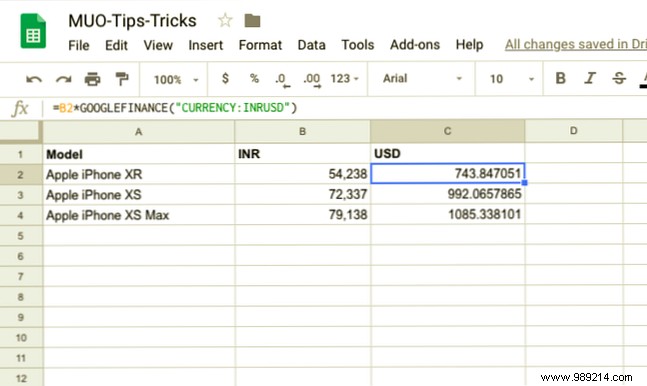
As an example, let us convert the price in India (in INR) of the latest iPhones to USD. So the syntax is formed as follows:
= B2 * GOOGLEFINANCE ("MONEDA: INRUSD")Be sure not to use the actual currency symbol, and instead stick to the three letter conventions.
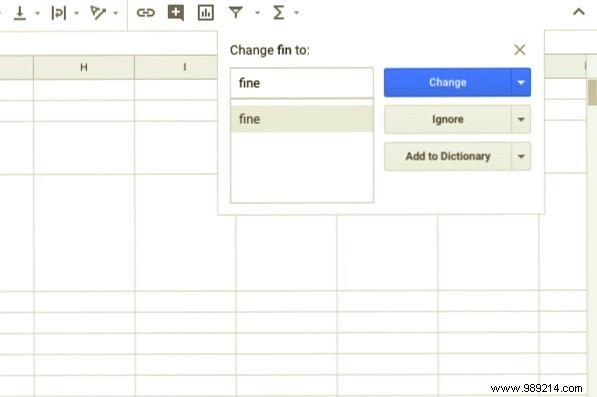
Spell Check is a daily feature that helps you keep your spreadsheet free of misspellings and typos. Manual spell checking is tedious. In such cases, it's always best to rely on Google's built-in spell checking feature and manually correct any discrepancies.
Here is how you can enable spell checker in google sheet,
As a precaution, it is not wise to rely entirely on the Spell Check feature. So make sure to give it a second look before the change.
Thanks to the Internet, international borders have been reduced. Just imagine this, you have just received a quote in a foreign language. Translating each cell will involve a lot of donkey work. Google Sheets has you covered with Translate function.
The Google Translate feature is capable of translating the content of hundreds of cells into multiple languages. Additionally, this feature will also help you detect which language is currently being used in Google Sheets. This is how you can translate individual cells in a spreadsheet from one language to another.
Use the following syntax:
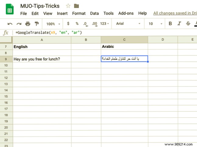
= GOOGLETRANSLATE (, "source_language", "target_language") Example:
= GOOGLETRANSLATE (A9, "en", "ar")In the example above, we have translated text (“Hey are you free for lunch”) from English to Arabic. If you don't mention the "target language", Google will automatically convert the cell to the default language.
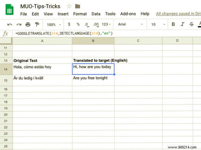
Google offers a nifty trick if you don't know the source language. In the above syntax, “source language” is replaced with “DETECT LANGUAGE ” and Sheets will automatically detect the source language and translate the cell to the language of your choice.
Use the following syntax:
= GOOGLETRANSLATE (A14, DETECTLANGUAGE (A14), "en")As part of this syntax, the language in cell. “A14” It is automatically detected and translated into the “Target Language” (English in this case). From GOOGLE TRANSLATE The function in Google Sheets is not an array function, you can simply drag the result and translate other cells as well.
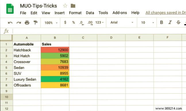
Heat mapping involves representing data in the form of a map where data values are represented as colors. Heatmaps are particularly popular in scientific studies when a large amount of data is collected and scientists create a heatmap to identify trends and patterns.
Thanks to the power of conditional formatting, you can easily create a heat map in Google Sheets. Follow the steps below to create a heatmap of your data
Note: The Google Sheets conditional formatting panel will also allow you to set the minimum or maximum values. Once this is done, the heatmap will stretch to values above the minimum, while those below the minimum will share the same color tone.
Copy pasting web data into your Google Sheets isn't exactly intuitive and effortless. There is a high probability that this could end up being a messy affair, especially if the dataset is large. Fortunately, Google Sheets lets you crawl websites. How to Build a Basic Web Crawler to Extract Information from a Website How to Build a Basic Web Crawler to Extract Information from a Website Have you ever wanted to capture information from a website? You can write a crawler to browse the website and extract only what it needs. Read More The best part is that you don't have to be a programmer to do this.
Let's see how the Google Sheets web scraper works with a live example.
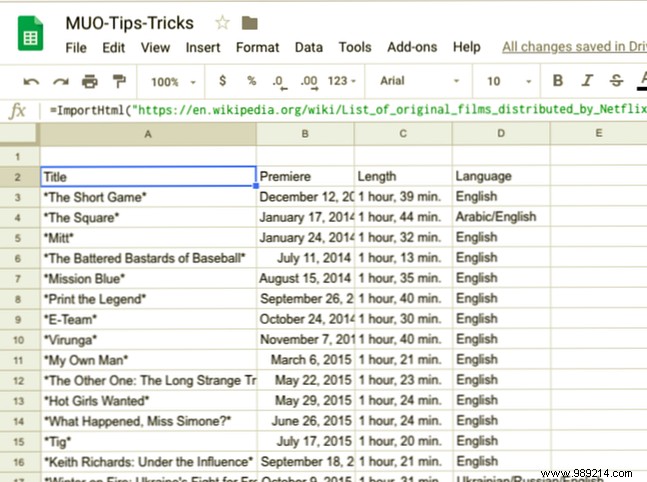
For the sake of demonstration, let's consider a Wikipedia page. This particular page is titled “List of Original Movies Distributed by Netflix.” and features multiple tables in different categories. I am interested in the documentary section. Use the ImportHTML syntax to dispose of the web page.
Use the following syntax:
= IMPORTHTML (URL, consulta, índice)The URL in this syntax corresponds to the address of this web page:
“https://en.wikipedia.org/wiki/List_of_original_films_distributed_by_Netflix” in our case.
The query is the part where you mention the item you intend to import, in our case the import item in the table. As you may have already noticed, the Wikipedia page features several tables. The argument called index is a way to specify which table you want to import.
In this case, it is Table 4. Finally, the syntax says the following:
= IMPORTHTML ("https://en.wikipedia.org/wiki/List_of_original_films_distributed_by_Netflix", "table", 4)And look! Google Sheets will automatically fetch the table from the Wikipedia page and the formatting won't be frustrated either.
Google Sheets is a universe of its own. Online web tools offer a host of features that can be leveraged to make your life easier. It's not just about productivity, as the quality of your data will also improve.
And for all this to happen, you don't need to be a computer geek. I personally prepare Google Sheets with the help of different templates. Try Google Sheets to Automatically Send an Invoice Every Month How to Automatically Send Monthly Invoices from Google Sheets How to Automatically Send Monthly Invoices from Google Sheets Do you regularly forget to send invoices? Here's how to automate the process with a Google script, or even a macro. Learn more or just automate repetitive tasks How to automate repetitive tasks in Google Sheets with macros How to automate repetitive tasks in Google Sheets with macros Macros are finally available to Google Sheets users. You don't need any coding knowledge to automate repetitive tasks in documents and spreadsheets. Read more . The possibilities are endless.