Microsoft Excel is a vibrant tool that is used for both business and personal tasks. How to Use Microsoft Excel to Manage Your Life How to Use Microsoft Excel to Manage Your Life It's no secret that I'm a total fan of Excel. A lot of that comes from the fact that I enjoy writing VBA code, and Excel combined with VBA scripts opens up a whole world of possibilities... Read More One robust feature is called conditional formatting. This feature can be useful for everyday situations as well as work-related ones. But, it can also be overwhelming if you've never used it.
Here are some general uses for conditional formatting, how to set them up, and of course what exactly this feature is capable of.
This wonderful feature of Excel applies formatting to cells based on the data filled in. Whether you're entering a number, percentage, letter, formula 16 Excel Formulas to Help You Solve Real Life Problems 16 Excel Formulas to Help You Solve Real Life Problems The right tool is half the work. Excel can solve calculations and process data faster than your calculator can. We show you the key Excel formulas and show you how to use them. Read More
For example, if you want the cell to highlight red every time you enter the letter A, this is a simple setup.
The tool has a variety of settings, options, and rules that can save time in detecting important items. And, for those familiar with the feature, it can be used quite a bit. However, it can also be advantageous for daily tasks at school, home, work and personal activities and for those who have never used it before.
Whether you're in high school or college, you can keep track of your assignments, due dates, and grades in Excel. With a couple of convenient conditional formatting options, you can quickly see important elements at a glance.
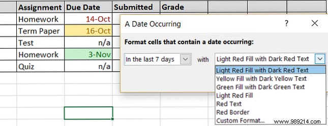
For due dates, you can apply formatting in a variety of ways to highlight what's due, due tomorrow, or due next month. It only takes a couple of steps:
This will help you see those important dates in a quick and easy way. Assignments due or due tomorrow will go out immediately.
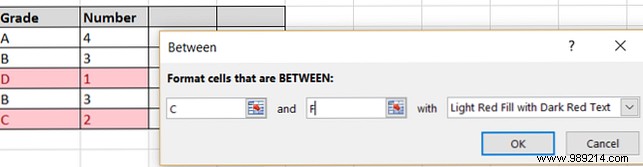
To keep track of grades and easily spot your lowest grades, you can apply formatting for letter and number grades that include a range.
This gives you a nice and easy way to see how well your classes are going and where your lowest grades are.
Excel's conditional formatting can be just as useful if you use the app at home. For finances, home projects, and to-do lists 10 Incredibly Useful Spreadsheet Templates to Organize Your Life 10 Incredibly Useful Spreadsheet Templates to Organize Your Life Is your life a hotbed of missed dates, forgotten purchases, and reneged commitments? ? Sounds like you need to get organized. Read More
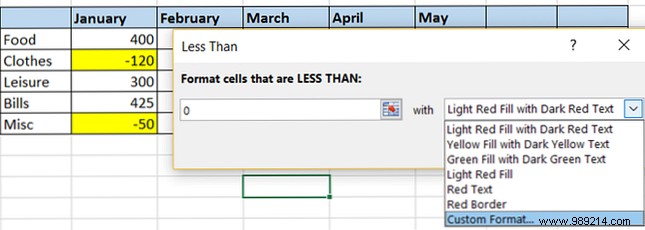
If you use it for your monthly budget, for example, you can spot problems quickly. Whether you've created your own spreadsheet or are using a handy template, it's helpful to format negative numbers automatically.
This provides a quick method of seeing negative numbers within your budget. And remember, you can apply any type of formatting that makes it more visible, from highlighting to text to border color.
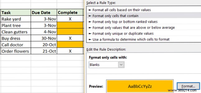
Excel is also a popular tool for to-do lists, and there's no better way to see what items you have that you haven't completed than with automatic formatting. With this approach, any task that is not checked is completed with an X will be highlighted.
Applying this format takes only a minute and can be very useful for keeping track of tasks you have yet to complete.
Many people keep careful track of their personal goals. From training sessions to weight maintenance, counting calories, 10 Excel templates to track your health and fitness, 10 Excel templates to track your health and fitness. Read More
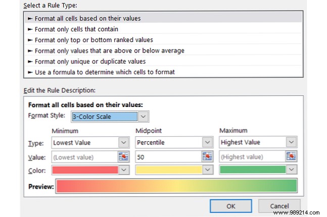
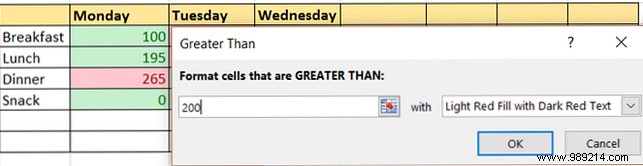
To count and track your calorie intake, apply the format to see when you go above and below your goal or limit for the day. In this case, we will apply two separate rules.
Then set the rule to go below the calorie limit.
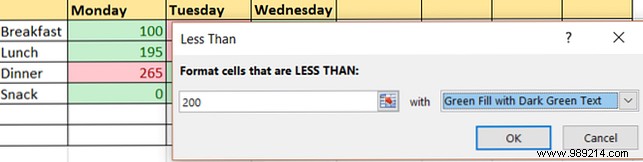
Note that in this example, if you enter the exact number 200 for the calorie count, no formatting will be applied. This is because the number does not fall under any rule.
For those who work remotely or as independent contractors, Excel can be used for tasks like time tracking or project estimates.
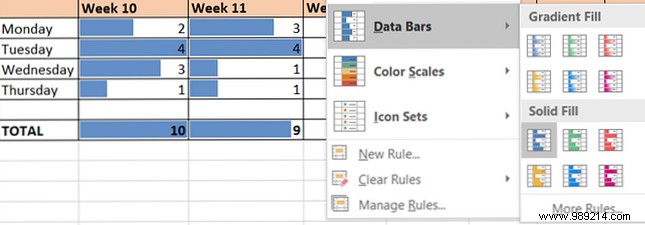
With a convenient way to track hours worked and view a summary for the week or month, the data bar format can be very helpful.
Once you enter the numbers in the designated cells, you will see the data bar adjust. The smaller the number, the smaller the bar and vice versa. You can also apply formatting to the totals you've calculated at the bottom. This is a good way to see your heaviest and lightest workdays, weeks or months.
Another great use of conditional formatting for business is to manage projects. 10 Useful Excel Project Management Templates for Tracking. 10 Useful Excel Project Management Templates for Tracking. Project management templates can help you replicate successful projects. Here are the essential Microsoft Excel templates for you. Read more . Using indicator shapes and highlighting for things like priority and effort can be beneficial, especially when sharing the information with others.
To set priorities using numbers with 1 as the highest priority in red and 3 as the lowest in green, you can apply shape formatting.
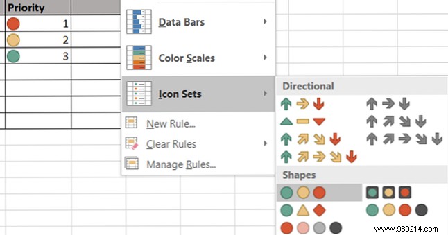
Now by entering the numbers 1, 2 and 3, you will see how the shapes adjust to their color. 3 Crazy Excel Formulas That Do Amazing Things 3 Crazy Excel Formulas That Do Amazing Things Conditional formatting formulas in Microsoft Excel can do amazing things. Here are some Excel formula productivity hacks. Read more . Note that if you use more than three numbers, which equals all three shapes, they will change accordingly. For example, 1 will remain red, while 2 and 3 will turn yellow, and 4 will be green. You can also reverse the order of shapes and assign specific numbers by selecting Conditional Formatting> Icon Sets> More Rules .
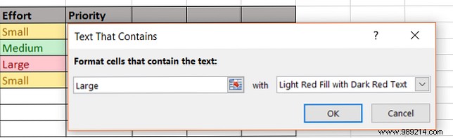
To set the effort for a project or task, you can format it using a specific word such as small, medium, or large.
Con este tipo de configuración de reglas, todo lo que tiene que hacer es escribir una palabra y la celda se formateará automáticamente para usted. Esto hace que ver los esfuerzos de su proyecto o tarea con una mirada sea extremadamente fácil.
¿Has probado el formato condicional para las actividades diarias? ¿O estás listo para comenzar a divertirte con esta función??
Comparte tus opiniones con nosotros en los comentarios a continuación.!