A pie chart is a wonderful tool for displaying information visually A printable chart for any occasion A printable chart for any occasion Charts are fantastic educational resources, they can help you stay organized, and if you pick a good one, they look amazing on your wall. Any board you need, you'll find something here. Read more . It allows you to see the data relationship with a whole pie, piece by piece. Also, if you use Microsoft Excel to track, edit, and share your data, the next logical step is to create a pie chart.
Using a simple spreadsheet of information, we'll show you how to make a useful pie chart. And once you get the hang of it, you can explore options using more data. How to Create Powerful Charts and Charts in Microsoft Excel How to Create Powerful Charts and Charts in Microsoft Excel A good chart can make the difference between making your point or leaving it. everybody snoozing We show you how to create powerful charts in Microsoft Excel that engage and inform your audience. Read more.
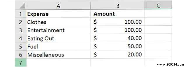
The most important aspect of your pie chart is the information. If you import a spreadsheet or create one from scratch, you must format it correctly for the chart. A pie chart in Excel can convert a row or column of data.
The Microsoft Office support website describes when a pie chart works best:
Keep in mind that with every change you make to your data, that pie chart updates in a handy and convenient way.
You can create a pie chart based on your data in two different ways, both of which start with selecting the cells. Be sure to select only the cells that need to be converted to the chart.
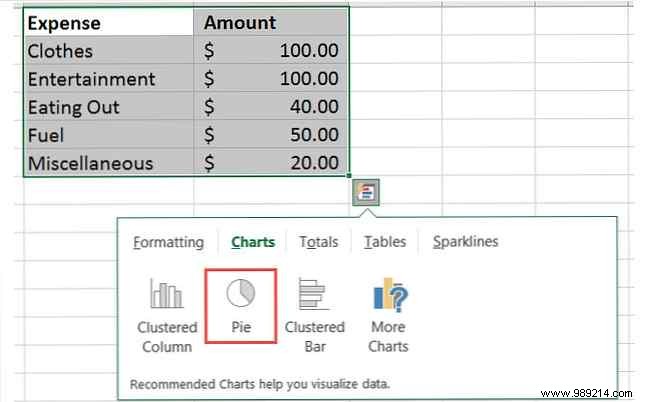
Select the cells, right click on the chosen group and select Quick Analysis from the context menu. Below Cards , you will choose Tart and you can preview it by hovering your mouse over it before clicking on it. Once you click on the pie chart, this will insert a basic style into your spreadsheet.
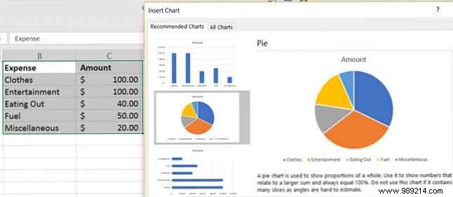
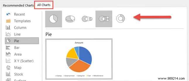
Select the cells, click the Insert and click the small arrow on the Chart Section of the tape to open it. You can see a pie chart in the Recommended Charts tab, but if not, click the All Cards tab and select Cake .
Before clicking OK to insert your table, you have a few options for styling. You can choose a basic cake, a three-dimensional cake, a cake tart, a cake bar, or a donut. After making your choice, click OK and the table will appear in your spreadsheet.
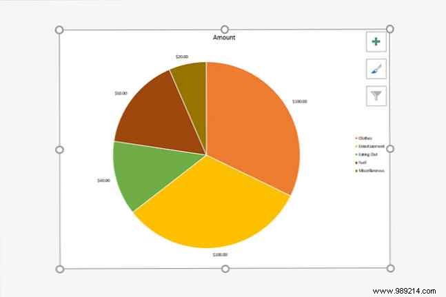
Once you have your pie chart in your spreadsheet, you can change things like the title, labels, and legend. You can also easily adjust colors, style, and general formatting or apply filters.
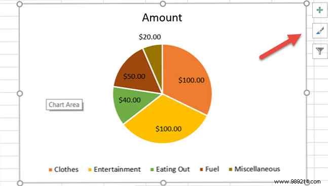
To start any change, click on the pie chart to display the three squares menu on the right.
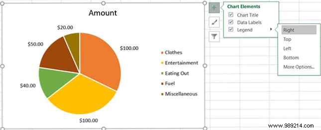
With the first menu option, you can adjust the chart title, data labels, and legend with various options for each. You can also decide whether or not to show these elements with the checkboxes.
To access each of the following elements, click on the chart, select Chart Elements , and then make your selection.
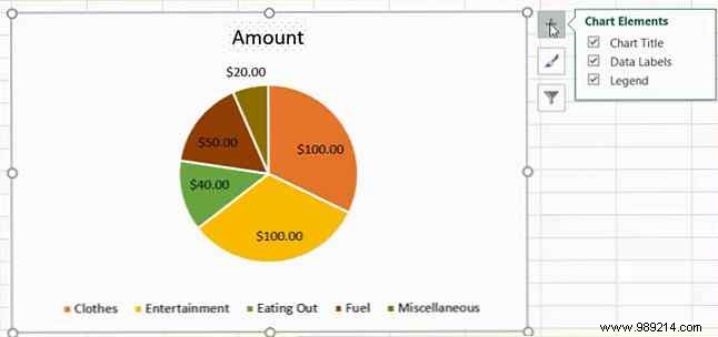
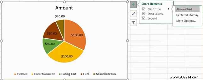
Chart title
If you want to adjust the title, select the arrow next to Chart title in the menu. You can choose to have the title on top of the chart or as a centered overlay.
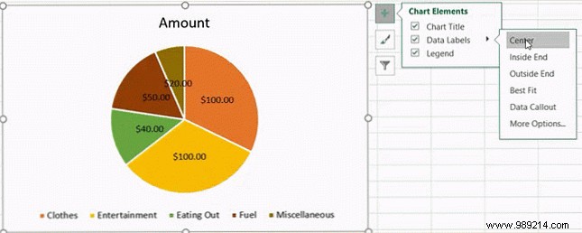
Data labels
To change labels, select the arrow next to Data Labels in the menu Then you can choose from five different locations on the chart for your labels to display.
Legend
As with the other elements, you can change where the legend is displayed. Select the arrow next to Legend in the menu Then you can choose to display the legend on any of the four sides of your chart.
More options
If you choose More options For any of these elements, a sidebar will open where you can add a fill color, border, shadow, glow, or other text options. You can also format the chart areas within the sidebar by clicking the arrow below Format Chart Area title.

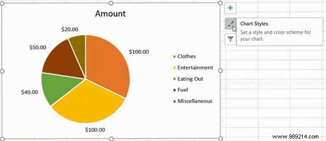
You can change the style and color scheme for your chart from numerous options.
To access each of the following elements, click on the chart, select Chart Styles , and then make your selection.
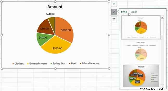
Style
Maybe you'd like to add patterns to the cutouts, change the background color, or have a simple two-tone graphic. With Excel, you can choose from 12 different styles of pie charts. Hover over each style for a quick preview.
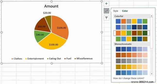
Colour
You can also choose from many color schemes for your pie chart. The Graphic style The menu shows colorful and monochrome options in the Color section. Again, use your mouse to preview each one.
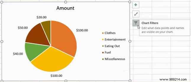
You may come across times when you would like to see only specific parts of the pie or hide names in the data series. This is when chart filters come in handy.
To access each of the following options, click the box, select Graphic Filters , and then make your selection.
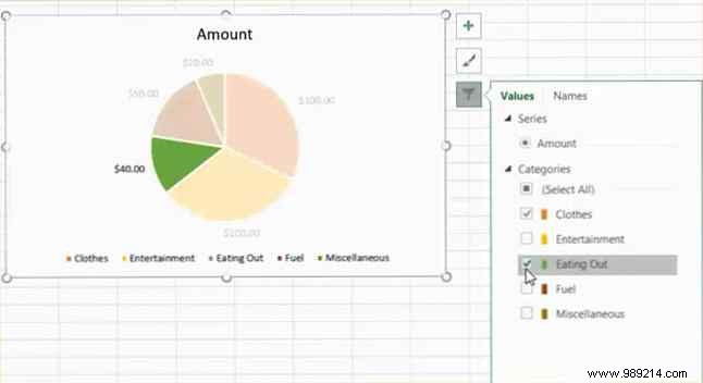
Valores
Asegúrate de estar en el Valores y luego marque o desmarque las casillas de las categorías que desea mostrar. Cuando termine, haga clic en Aplicar .
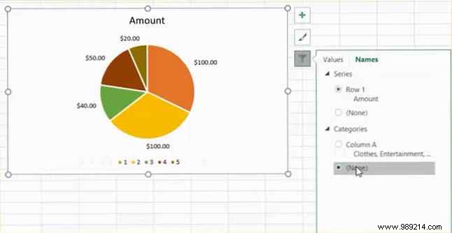
Los nombres
Si desea cambiar la visualización del nombre, haga clic en Los nombres section. Luego, marque el botón de opción para sus selecciones para las series y categorías y haga clic en Aplicar When you're done.
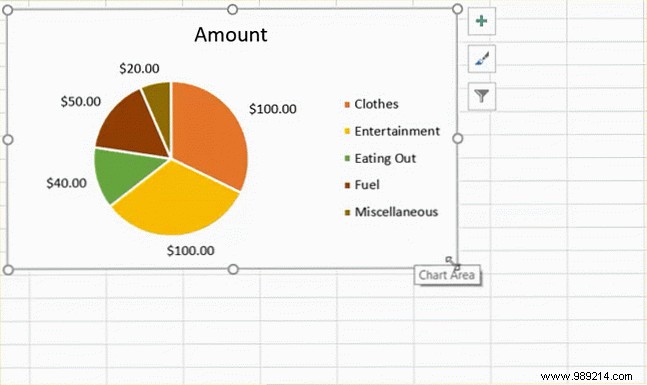
Cuando crees tu gráfico, Excel lo dimensionará y lo colocará en tu hoja de cálculo en un lugar abierto. Sin embargo, puede cambiar su tamaño, arrastrarlo a otro lugar o moverlo a otra hoja de cálculo..
Haga clic en su gráfico circular y cuando aparezcan los círculos en el borde del gráfico, puede tirar para cambiar el tamaño. Asegúrese de que la flecha que ve en el círculo cambie a una flecha de dos vías .
Una vez más, haga clic en su gráfico circular y con la flecha de cuatro lados que se muestra, arrástrelo a su nuevo punto en la hoja de cálculo.

Si desea mover el gráfico a otra hoja de cálculo, puede hacerlo fácilmente. Haga clic derecho en el gráfico y seleccione Mover gráfico from the context menu. Entonces, recoger Objeto en y selecciona tu hoja en la ventana emergente.
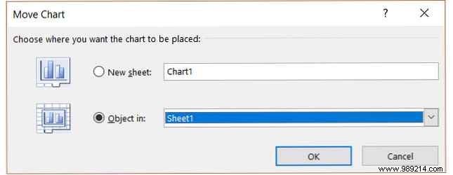
También puede crear una nueva hoja para el gráfico que se mostrará bien sin filas ni columnas de la hoja de cálculo. Seleccionar Hoja nueva e ingrese un nombre en la ventana emergente.
Si desea incluir su gráfico circular de Excel en una presentación de PowerPoint Mejore su presentación de PowerPoint con visualizaciones de datos de Excel Mejore su presentación de PowerPoint con visualizaciones de datos de Excel Nada hace que la información sea más vívida que una excelente visualización. We show you how to prepare your data in Excel and import the charts into PowerPoint for an animated presentation. Leer más, esto se hace fácilmente con la acción de copiar y pegar.
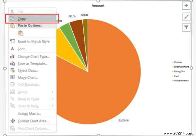
En Excel, seleccione el gráfico y luego haga clic en Dupdo desde el Casa pestaña o haga clic derecho y seleccione Dupdo desde el menú contextual.
A continuación, abra PowerPoint y navegue a la diapositiva donde desea el gráfico. Haga clic en la diapositiva y seleccione Pegar desde el Casa pestaña o haga clic derecho y elija Pegar desde el menú contextual.
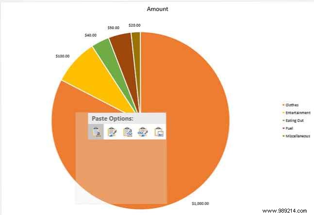
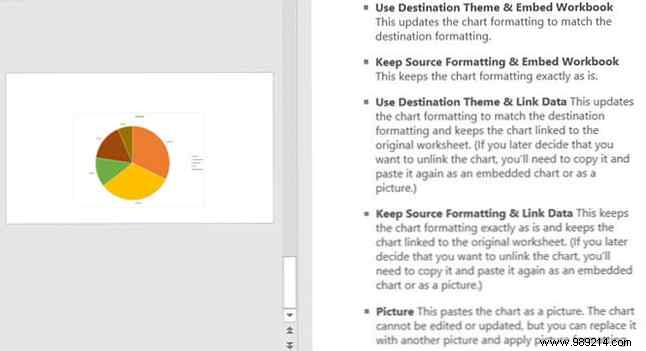
Tenga en cuenta que tiene diferentes opciones de pegado en las aplicaciones de Microsoft Office. Puede pegar con el formato de destino o de origen, cada uno con datos incrustados o vinculados. O simplemente pegarlo como una imagen.
La creación inicial de un gráfico circular en Excel es más simple de lo que probablemente se piensa. Y si disfruta experimentando con diferentes estilos, estilos y colores que se adaptan a su negocio, es muy fácil. Excel ofrece una variedad de opciones para que usted cree un gráfico circular que se adapte a sus necesidades y preferencias.
¿Ya ha creado un gráfico circular en Excel o es la primera vez que lo hace? 8 Consejos para saber cómo aprender Excel rápidamente 8 Consejos para saber cómo aprender Excel rápidamente ¿No está tan cómodo con Excel como quisiera? Get started with simple tips for adding formulas and managing data. Follow this guide and you'll be up to speed in no time. Read more ? ¿Cuál es tu característica favorita para perfeccionar tu carta? Háganos saber sus pensamientos!