Microsoft Excel is a premier application for anyone who has to work with a lot of numbers, from students to accountants. But its usefulness extends beyond large databases Excel Vs. Access:Can a spreadsheet replace a database? Excel Vs. Access:Can a Spreadsheet Replace a Database? Which tool should I use to manage the data? Access and Excel both have data filtering, compiling, and querying. We will show you which one is the most suitable for your needs. Read more; You can also do a lot of great things with text. The functions listed below will help you parse, edit, convert, and make changes to text, saving you many hours of boring and repetitive work.
This guide is available to download as a free PDF. Download Save Time with Text Operations in Excel Now . Feel free to copy and share this with your friends and family.Navigation:Non-destructive editing | Half-width and full-width characters | Character Features | Text Analysis Features | Text conversion features | Text editing features | Text replacement functions | Text Die Cutting Features | A real world example
One of the principles of using Excel's text functions is non-destructive editing. In a nutshell, this means that whenever you use a function to make a change to text in a row or column, that text will remain unchanged and the new text will be placed in a new row or column. This can be a bit disorienting at first, but can be invaluable, especially if you're working with a large spreadsheet that would be difficult or impossible to rebuild if an edit goes wrong.
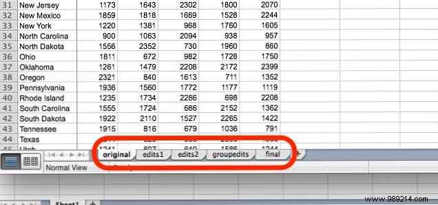
While you can continue to add columns and rows to your ever-expanding giant spreadsheet, one way to take advantage of this is to save your original spreadsheet on the first sheet of a document and the edited copies on other sheets. That way, no matter how many edits you make, you'll always have the original data you're working with.
Some of the functions discussed here refer to single-byte and double-byte character sets, and before we begin, it will be helpful to clarify exactly what these are. In some languages, such as Chinese, Japanese, and Korean, each character (or a number of characters) will have two possibilities to be displayed:one is encoded in two bytes (known as a full-width character), and one is encoded in A single byte (half width). You can see the difference in these characters here:
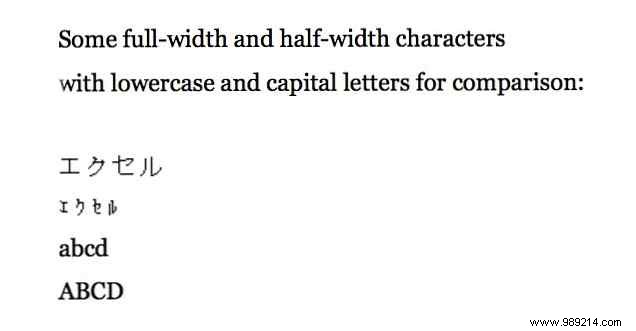
As you can see, double-byte characters are larger and often easier to read. However, in some computing situations, one or another of these types of encodings is required. If you don't know what this means or why you should care, chances are you don't need to think about it. In case you do, however, there are features included in the following sections that relate specifically to half-width and full-width characters.
It's not very often that you work with individual characters in Excel, but such situations do arise from time to time. And when they do, these features are the ones you need to know about.
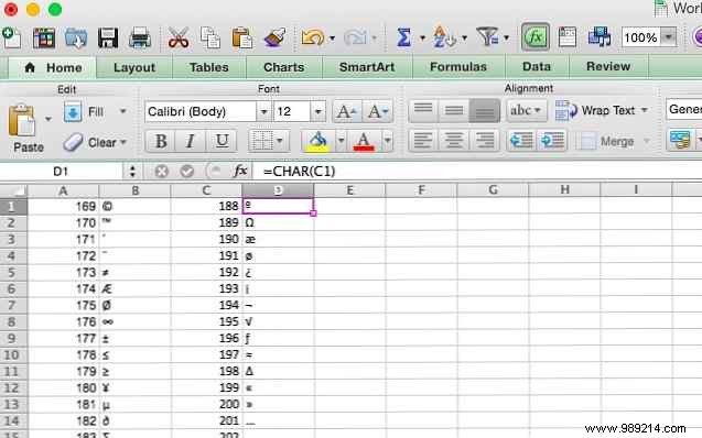
CHAR takes a character number and returns the corresponding character; If you have a list of numbers of characters, for example, CHAR will help you convert them to the characters you're most used to. The syntax is quite simple:
= CHAR ([texto])
[text] can take the form of a cell reference or a character; so =CHAR(B7) and =CHAR(84) both work. Note that when you use CHAR, it will use the encoding your computer is set to; so su =CHAR(84) might be different than mine (especially if you're on a Windows computer, since I'm using Excel for Mac).
If the number you are converting to is a Unicode character number and you are using Excel 2013, you will need to use the UNICHAR function. Earlier versions of Excel do not have this feature.
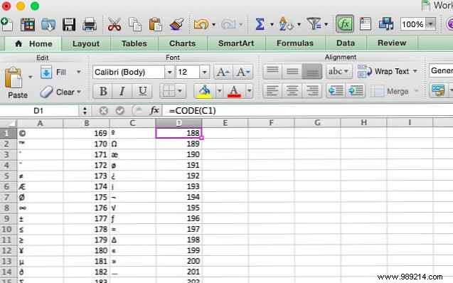
As you might expect, CODE and UNICODE do the exact opposite of the CHAR and UNICHAR functions:they take a character and return the number of the encoding you've chosen (or is set to the default value on your computer). It's important to note that if you run this function on a string that contains more than one character, it will only return the character reference for the first character in the string. The syntax is very similar:
= CÓDIGO ([texto])
In this case, [text] is a character or a string. And if you want the Unicode reference instead of your computer's default, it will use UNICODE (again, if you have Excel 2013 or later).
The functions in this section will help you get information about the text in a cell, which can be useful in many situations. We'll start with the basics.
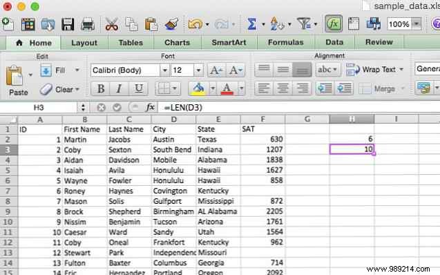
LEN is a very simple function:it returns the length of a string. So if you need to count the number of letters in a group of different cells, this is the way to go. Here is the syntax:
= LEN ([texto])
The [text] argument is the cell or cells you would like to count. You can see below that when using the LEN function on a cell containing the city name “Austin,” it returns 6. When used on the city name “South Bend,” it returns 10. A space counts as a character with LEN, so keep that in mind if you're using it to count the number of letters in a given cell.
The related LENB function does the same thing, but works with double-byte characters. If you were to count a string of four double-byte characters with LEN, the result would be 8. With LENB, it's 4 (if you have DBCS enabled as your default language).
You may wonder why you would use a function called FIND if you can just use CTRL + F or Edit> Find. The answer lies in the specificity with which you can search using this function; Instead of searching the entire document, you can choose which character in each string to start the search on. The syntax will help clarify this confusing definition:
= FIND ([find_text], [within_text], [start_num])
[find_text] is the string you are looking for. [within_text] is the cell(s) Excel will look in for that text, and [start_num] is the first character it will see. It is important to note that this function is case sensitive. Let's take an example.
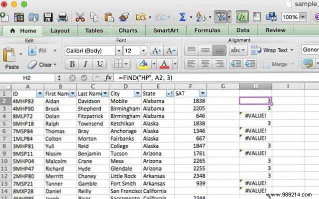
I have updated the sample data so that each student's ID number is an alphanumeric sequence of six characters, each beginning with a single digit, an M for "male," a two-letter sequence to indicate level of student achievement (HP for high, SP for standard, LP for low, and UP/XP for unknown) and a final sequence of two numbers. Let's use FIND to spotlight every high-achieving student. Here is the syntax we will use:
= ENCONTRAR ("HP", A2, 3) This will tell us if HP appears after the third character in the cell. Applied to all cells in the ID column, we can see at a glance whether or not the student was a top performer (note that the 3 returned by the function is the character HP is on). FIND may be better used if you have a wider variety of sequences, but you get the idea.
As with LEN and LENB, FINDB is used for the same purpose as FIND, only with double-byte character sets. This is important due to the specification of a certain character. If you are using a DBCS and you specify the fourth character with FIND, the search will start at the second character. FINDB solves the problem.
Note that FIND is case sensitive, so you can search for a specific capitalization. If you want to use a case-insensitive alternative, you can use the SEARCH function, which takes the same arguments and returns the same values.
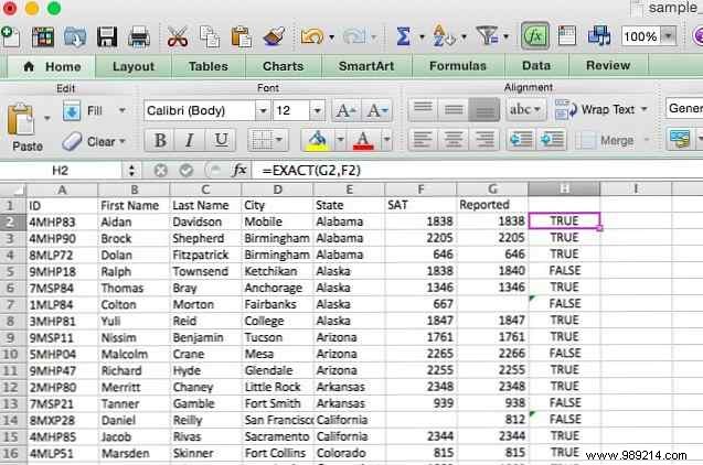
If you need to compare two values to see if they are equal, EXACT is the function for you. When you supply EXACT with two strings, it will return TRUE if they are exactly the same, and FALSE if they are different. Because EXACT is case sensitive, it will return FALSE if you give it strings that read “Test” and “test.” Here is the EXACT syntax:
= EXACTO ([texto1], [texto2])
Both arguments are pretty self-explanatory; are the strings you would like to compare. In our spreadsheet, we'll use them to compare two SAT scores. I have added a second row and called it. "Informed." We will now look at the spreadsheet with EXACT and see where the reported score differs from the official score using the following syntax:
= EXACTO (G2, F2)
Repeating that formula for each row in the column gives us this:
These functions take the values in a cell and convert them to another format; for example, from a number to a string or from a string to a number. There are a few different options on how to do this and what the exact result is.
TEXT converts numeric data to text and allows you to format it in specific ways; this could be useful, for example, if you plan to use Excel data in a Word document How to Integrate Excel Data into a Word Document How to Integrate Excel Data into a Word Document During your work week, there are probably many times that you find yourself copying and pasting information from Excel into Word, or the other way around. This is how people often produce written reports... Read More Let's look at the syntax and then see how you could use it:
= TEXTO ([texto], [formato])
The [format] argument allows you to choose how you want the number to appear in the text. There are several different operators you can use to format your text, but we'll stick to a simple one here (for more information, see the Microsoft Office help page on TEXT). TEXT is often used to convert monetary values, so we'll start with that.
I have added a column called “Enrollment” that contains a number for each student. We'll format that number into a string that looks a bit more like what we're used to reading monetary values for. Here is the syntax we will use:
= TEXTO (G2, "$ #, ###")
Using this format string will give us numbers that are preceded by the dollar sign and include a comma after the hundreds place. This is what happens when we apply it to the spreadsheet:
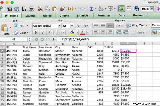
Each number now has the correct format. You can use TEXT to format numbers, currency values, dates, times, and even to remove insignificant digits. For details on how to do all of these things, see the help page linked above.
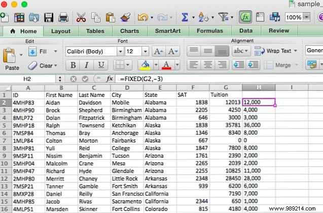
Similar to TEXT, the FIX function takes input and formats it as text; however, FIXED specializes in converting numbers to text and gives you some specific options for formatting and rounding the output. Here is the syntax:
= FIJO ([número], [decimales], [no_commas])
The [number] argument contains the reference to the cell you want to convert to text. [decimals] is an optional argument that allows you to choose the number of decimal places to retain in the conversion. If this is 3, you will get a number like 13,482. If you use a negative number for decimals, Excel will round the number. Let's take a look at that in the following example. [no_commas], if set to TRUE, will exclude commas from the final value.
We'll use this to round the tuition values we used in the last example to the nearest thousand.
= FIJO (G2, -3)
When applied to the row, we get a row of rounded license plate values:
This is the opposite of the TEXT function:it takes any cell and converts it to a number. This is especially useful if you import a spreadsheet or copy and paste a large amount of data and format it as text. Here's how to fix it:
= VALOR ([texto])
That's all about it. Excel will recognize the accepted formats of constant numbers, times, and dates, and convert them to numbers that can then be used with number functions and formulas. This one is pretty simple, so we skip the example.
Like the TEXT function, DOLLAR converts a value to text, but also adds a dollar sign. You can choose the number of decimal places to include, like this:
= DÓLAR ([texto], [decimales])
If you leave the [decimals] argument blank, the value defaults to 2. If you include a negative number for the [decimals] argument, the number will be rounded to the left of the decimal.
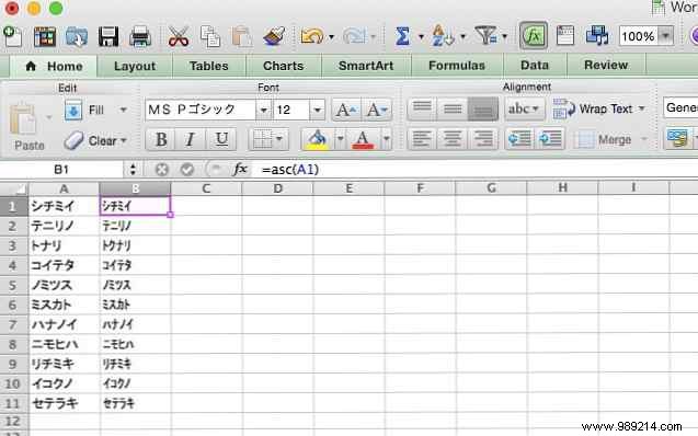
Remember our discussion about single-byte and double-byte characters? This is how it becomes between them. Specifically, this function converts full-width, double-byte characters to half-width, single-byte characters. It can be used to save space in the spreadsheet. Here is the syntax:
= ASC ([texto])
Pretty simple. Just run the ASC function on whatever text you want to convert. To see it in action, I'll convert this spreadsheet, which contains a number of Japanese katakana, which are often represented as full-width characters. Let's change them to half width.
Of course, if you can convert one way, you can also convert back the other way. JIS converts from half-width characters to full-width characters. Like ASC, the syntax is very simple:
= JIS ([texto])
The idea is pretty simple, so we'll move on to the next section without an example.
One of the most useful things you can do with text in Excel is to make changes to it programmatically. The following functions will help you take text input and get the exact formatting that is most useful to you.
These are all very simple functions to understand. UPPER makes the text uppercase, LOWER makes it lowercase, and RIGHT capitalizes the first letter of each word, while leaving all other letters lowercase. There's no need for an example here, so I'll just give you the syntax:
= SUPERIOR / INFERIOR / ADECUADO ([texto])
Choose the cell or range of cells that your text for the [text] argument is in, and you're ready to go.
Importing data into Excel usually goes pretty well, but sometimes you end up with characters you don't want. This is most common when there are special characters in the original document that Excel cannot display. Instead of going through all the cells that contain those characters, you can use the CLEAR function, which looks like this:
= LIMPIO ([texto])
The [text] argument is simply the location of the text you want to clean. In the example spreadsheet, I've added some non-printable characters to the names in Column A that need to be removed (there's one in row 2 that pushes the name to the right, and an error character in row 3). I have used the CLEAR function to transfer the text to Column G without those characters:
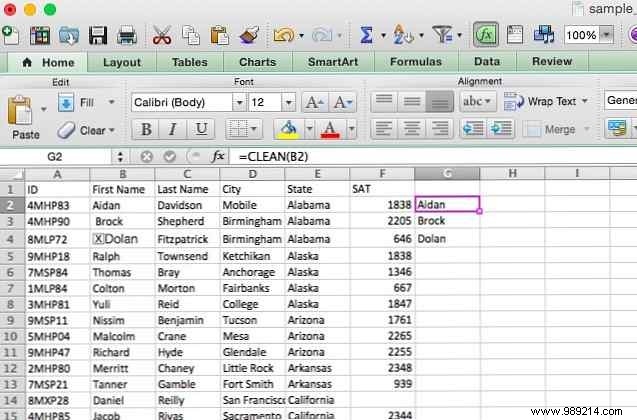
Column G now contains the names without the non-printing characters. This command is not only useful for text; it can often help you if the numbers are messing up your other formulas as well; Special characters can really wreak havoc on calculations. It's essential when you're converting from Word to Excel Convert Word to Excel - Turn your Word document into an Excel file Convert Word to Excel - Turn your Word document into an Excel file Read More.
While CLEAN removes non-printing characters, TRIM removes extra spaces at the beginning or end of a text string that you might end up with these if you copy text from Word or a plain text document and it ends with something like "Track Date" ... convert it to “Follow Up Date,” just use this syntax:
= TRIM ([texto])
When you use it, you will see results similar to when you use CLEAN.
Occasionally you will need to replace specific strings in your text with a string of other characters. Using Excel formulas is much faster than find and replace Conquer 'Find and Replace' text tasks with wReplace Conquer 'Find and Replace' text tasks with wReplace Read More .
If you're working with a lot of text, sometimes you'll need to make some big changes, like replacing one text string with another. Perhaps you realized that the month is wrong on a series of bills. Or that you spelled someone's name incorrectly. In any case, it is sometimes necessary to replace a string. That's what SUBSTITUTE is for. Here is the syntax:
= SUSTITUTO ([texto], [texto antiguo], [texto nuevo], [instancia])
The [text] argument contains the location of the cells you want to replace in, and the [oldtext] and [text_text] are self-explanatory. [instance] allows you to specify a specific instance of the old text to replace. So if you want to replace only the third instance of the old text, you must enter "3" for this argument. SUBSTITUTE will copy over all other values (see below).
As an example, we will correct a spelling error in our spreadsheet. Digamos “Honolulu” fue escrito accidentalmente como “Honululu.” Aquí está la sintaxis que usaremos para corregirla:
= SUSTITUTO (D28, "Honululu", "Honolulu")
Y esto es lo que sucede cuando ejecutamos esta función:
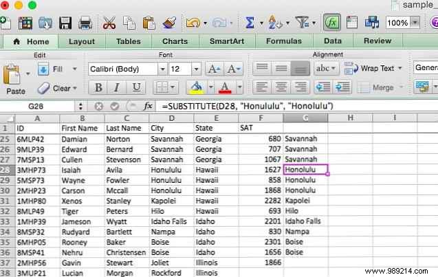
Después de arrastrar la fórmula a las celdas circundantes, verás que todas las celdas de la columna D se copiaron, excepto las que contenían el error ortográfico. “Honululu,” que fueron reemplazados con la ortografía correcta.
REPLACE es muy similar a SUBSTITUTE, pero en lugar de reemplazar una cadena de caracteres específica, reemplazará a los personajes en una posición específica. Un vistazo a la sintaxis dejará claro cómo funciona la función:
= REEMPLAZAR ([old_text], [start_num], [num_chars], [new_text])
[old_text] es donde especificará las celdas en las que desea reemplazar el texto. [start_num] es el primer carácter que le gustaría reemplazar, y [num_chars] es el número de caracteres que se reemplazarán. Veremos cómo funciona esto en un momento. [new_text], por supuesto, es el nuevo texto que se insertará en las celdas; esto también puede ser una referencia de celda, que puede ser bastante útil.
Echemos un vistazo a un ejemplo. En nuestra hoja de cálculo, las ID de los estudiantes tienen secuencias de HP, SP, LP, UP y XP. Queremos deshacernos de ellos y cambiarlos todos a NP, lo que llevaría mucho tiempo usando SUSTITUIR o Buscar y reemplazar. Aquí está la sintaxis que usaremos:
= REEMPLAZAR (A2, 3, 2, "NP")
Aplicado a toda la columna, esto es lo que obtenemos:
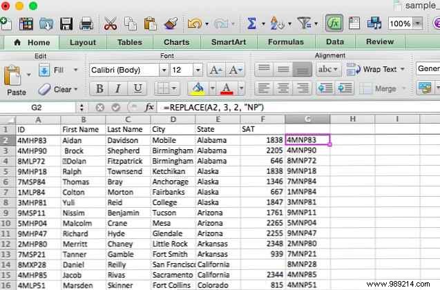
Todas las secuencias de dos letras de la Columna A han sido reemplazadas por “notario público” en la columna G.
Además de hacer cambios en las cuerdas, también puedes hacer cosas con piezas más pequeñas de esas cuerdas (o usar esas cuerdas como piezas más pequeñas para formar las más grandes). Estas son algunas de las funciones de texto más utilizadas en Excel..
Este es uno que yo mismo he usado varias veces. Cuando tiene dos celdas que deben agregarse juntas, CONCATENAR es su función. Aquí está la sintaxis:
= CONCATENAR ([texto1], [texto2], [texto3]…)
Lo que hace que la concatenación sea tan útil es que los argumentos [texto] pueden ser de texto plano, como “Arizona,” o referencias de celdas como “A31.” Incluso puedes mezclar los dos. Esto le puede ahorrar una gran cantidad de tiempo cuando necesita combinar dos columnas de texto, como si necesita crear un “Nombre completo” columna de un “Nombre de pila” y un “Apellido” columna. Aquí está la sintaxis que usaremos para hacer eso:
= CONCATENADO (A2, "", B2)
Observe aquí que el segundo argumento es un espacio en blanco (escrito como quotation-mark-space-qoutation-mark). Sin esto, los nombres se concatenarían directamente, sin espacio entre el nombre y los apellidos. Veamos qué sucede cuando ejecutamos este comando y usamos autocompletar en el resto de la columna:
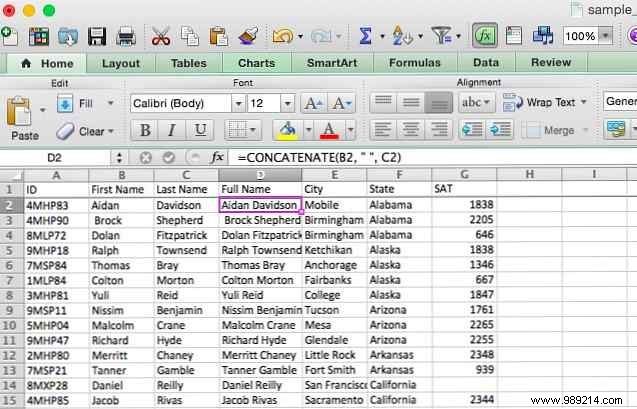
Ahora tenemos una columna con el nombre completo de todos. Puede usar fácilmente este comando para combinar códigos de área y números de teléfono, nombres y números de empleados, ciudades y estados, o incluso signos y montos de moneda.
Puede acortar la función CONCATENAR a un solo símbolo en la mayoría de los casos. Para crear la fórmula anterior usando el signo, deberíamos escribir esto:
= A2 & "" & B2
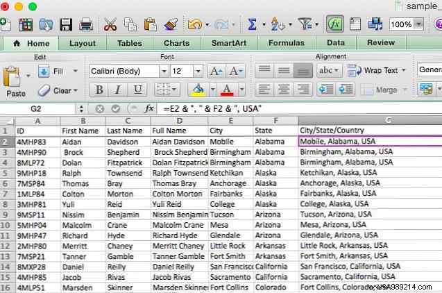
También puedes usarlo para combinar referencias de celdas y líneas de texto, como esto:
= E2 & "," & F2 & ", EE. UU."
Esto toma las celdas con nombres de ciudades y estados y las combina con “Estados Unidos” para obtener la dirección completa, como se ve a continuación.
A menudo, desea trabajar solo con los primeros (o últimos) pocos caracteres de una cadena de texto. IZQUIERDA y DERECHA le permiten hacerlo devolviendo solo un cierto número de caracteres que comienzan con el carácter de la izquierda o la derecha de una cadena. Aquí está la sintaxis:
= IZQUIERDA / DERECHA ([texto], [num_chars])
[texto], por supuesto, es el texto original, y [num_chars] es el número de caracteres que desea devolver. Veamos un ejemplo de cuándo es posible que desee hacer esto. Digamos que ha importado varias direcciones, y cada una contiene la abreviatura del estado y el país. Podemos usar IZQUIERDA para obtener solo las abreviaturas, usando esta sintaxis:
= IZQUIERDA (E2, 2)
Esto es lo que se ve aplicado a nuestra hoja de cálculo:
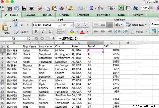
Si la abreviatura hubiera aparecido después del estado, habríamos usado RIGHT de la misma manera.
MID es muy parecido a IZQUIERDA y DERECHA, pero te permite sacar caracteres de la mitad de una cadena, comenzando en la posición que especifiques. Echemos un vistazo a la sintaxis para ver exactamente cómo funciona:
= MID ([texto], [start_num], [num_chars])
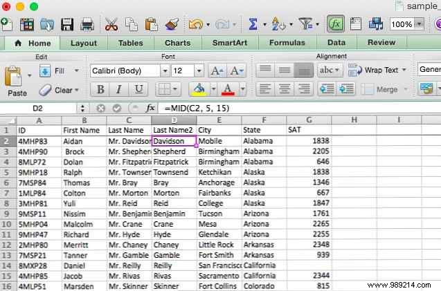
[start_num] es el primer carácter que se devolverá. Esto significa que si desea que el primer carácter de una cadena se incluya en el resultado de una función, esto será “1.” [num_chars] es el número de caracteres después del carácter inicial que se devolverá. Vamos a hacer un poco de limpieza de texto con esto. En la hoja de cálculo de ejemplo, ahora tenemos títulos agregados a los apellidos, pero nos gustaría eliminarlos para que un apellido de “Sr. Martin” será devuelto como “Martín.” Aquí está la sintaxis:
= MID (A2, 5, 15)
Nosotros usaremos “5” como el carácter inicial, porque la primera letra del nombre de la persona es el quinto carácter (“Señor. ” ocupa cuatro espacios). La función devolverá las siguientes 15 letras, que deberían ser suficientes para no cortar la última parte del nombre de nadie. Aquí está el resultado en Excel:
En mi experiencia, encuentro que MID es más útil cuando lo combinas con otras funciones. Digamos que esta hoja de cálculo, en lugar de incluir solo a los hombres, también incluye a las mujeres, que podrían tener “Sra.” o “señora.” por sus títulos. ¿Qué haríamos entonces? Puedes combinar MID con IF para obtener el primer nombre independientemente del título:
= IF (IZQUIERDA (A2, 3) = "Mrs", MID (A2, 6, 16), MID (A2, 5, 15)
Le dejaré averiguar exactamente cómo funciona esta fórmula. Es posible que tenga que revisar los operadores booleanos de Excel. Mini tutorial de Excel:usar la lógica booleana para procesar datos complejos. Tutorial de mini Excel:usar la lógica booleana para procesar datos complejos. Operadores lógicos SI, NO , Y, y O, pueden ayudarlo a pasar de un novato de Excel a un usuario avanzado. Le explicamos los conceptos básicos de cada función y le mostramos cómo puede usarlos para obtener los máximos resultados. Más información).
Si necesitas tomar una cadena y repetirla varias veces, y prefieres no escribirla una y otra vez, REPT puede ayudarte. Dar a REPT una cadena (“a B C”) y un número (3) de veces que desea que se repita, y Excel le dará exactamente lo que pidió (“abcabcabc”). Aquí está la sintaxis muy fácil:
= REPT ([texto], [número])
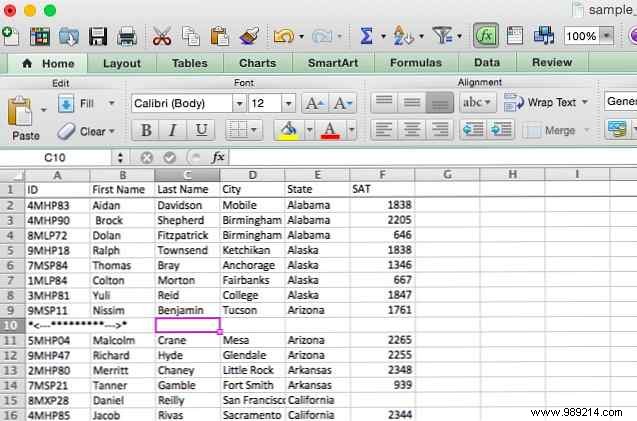
[texto], obviamente, es la cadena base; [número] es el número de veces que desea que se repita. Aunque todavía no he encontrado un buen uso de esta función, estoy seguro de que alguien podría usarlo para algo. Usaremos un ejemplo que, si bien no es exactamente útil, podría mostrarle el potencial de esta función. Vamos a combinar REPT con “Y” para crear algo nuevo. Aquí está la sintaxis:
= "*<---" & REPT("*", 9) & "--->* " El resultado se muestra a continuación:
Para darle una idea de cómo podría poner una función de texto en uso en el mundo real, le daré un ejemplo de dónde combiné MID con varios condicionales en mi propio trabajo. Para mi posgrado en psicología, realicé un estudio en el que los participantes tenían que hacer clic en uno de los dos botones y se registraron las coordenadas de ese clic. El botón a la izquierda de la pantalla estaba etiquetado como A, y el de la derecha estaba etiquetado como B. Cada prueba tenía una respuesta correcta, y cada participante hizo 100 pruebas.
Para analizar estos datos, necesitaba ver cuántos ensayos acertó cada participante. Así es como se veía la hoja de cálculo de resultados, después de un poco de limpieza:
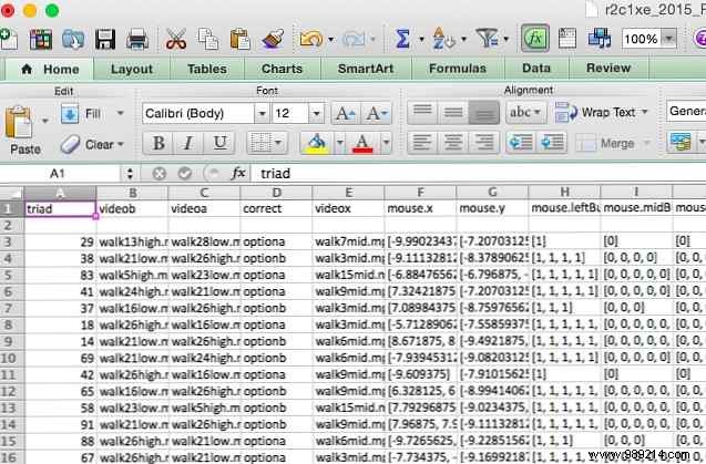
La respuesta correcta para cada prueba se incluye en la columna D, y las coordenadas del clic se enumeran en las columnas F y G (están formateadas como texto, lo cual es un asunto complicado). Cuando empecé, simplemente pasé e hice el análisis manualmente; si la columna d dijo “opciona” y el valor en la columna F era negativo, ingresaría 0 (para “incorrecto”). Si fuera positivo, ingresaría 1. Lo contrario era cierto si la columna D decía:“opcionb.”
Después de un poco de retoques, se me ocurrió una forma de usar la función MID para hacer el trabajo por mí. Esto es lo que usé:
= IF (D3 = "optiona", IF (MID (F3,2,1) = "-", 1,0), IF (MID (F3,2,1) = "-", 0,1))
Vamos a romper eso. Comenzando con la primera declaración IF, tenemos lo siguiente:“si la celda D3 dice 'optiona', entonces [primer condicional]; si no, entonces [segundo condicional].” El primer condicional dice esto:“si el segundo carácter de la celda F3 es un guión, devuelva verdadero; si no, devuelve falso.” El tercero dice “si el segundo carácter de la celda F3 es un guión, devuelva falso; si no, regresa verdadero.”
Podría tomar un tiempo envolver su cabeza alrededor de esto, pero debería quedar claro. En resumen, esta fórmula verifica si D3 dice “opciona”; si lo hace, y el segundo carácter de F3 es un guión, la función devuelve “cierto.” Si D3 contiene “opciona” y el segundo carácter de F3 no es un guión, vuelve “falso.” Si D3 no hace Contiene “opciona” y el segundo caracter de F3 es un guion, devuelve “falso.” Si D3 no dice “opciona” y el segundo carácter de F2 no es un guión, vuelve “cierto.”
Así es como se ve la hoja de cálculo cuando ejecutas la fórmula:
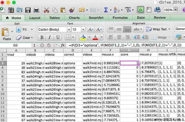
Ahora el “Puntuación” la columna contiene un 1 por cada prueba que el participante respondió correctamente y un 0 por cada prueba que respondieron incorrectamente. A partir de ahí, es fácil resumir los valores para ver cuántos acertaron..
Espero que este ejemplo le dé una idea de cómo puede usar creativamente las funciones de texto cuando trabaja con diferentes tipos de datos. El poder de Excel es casi ilimitado 3 fórmulas locas de Excel que hacen cosas increíbles 3 fórmulas locas de Excel que hacen cosas asombrosas Las fórmulas de formato condicional en Microsoft Excel pueden hacer cosas maravillosas. Here are some Excel formula productivity hacks. Lea más, y si se toma el tiempo de idear una fórmula que haga su trabajo por usted, puede ahorrar mucho tiempo y esfuerzo.!
Excel es una fuente de poder cuando se trata de trabajar con números, pero también tiene una sorprendente cantidad de funciones útiles de texto. Como hemos visto, puede analizar, convertir, reemplazar y editar texto, así como combinar estas funciones con otras para hacer cálculos y transformaciones complejas..
Desde el envío de correos electrónicos Cómo enviar correos electrónicos desde una hoja de cálculo de Excel mediante secuencias de comandos de VBA Cómo enviar correos electrónicos desde una hoja de cálculo de Excel mediante secuencias de comandos de VBA Nuestra plantilla de código lo ayudará a configurar correos electrónicos desde Excel utilizando Objetos de datos de colaboración (CDO) y secuencias de comandos de VBA. Leer más para hacer sus impuestos ¿Haciendo sus impuestos? 5 Excel formulas you should know doing your taxes? 5 Excel Formulas You Need to Know It's two days before your taxes are due and you don't want to pay another late filing fee. This is the time to harness the power of Excel to put everything in order. Lea más, Excel puede ayudarlo a administrar toda su vida. Cómo usar Microsoft Excel para administrar su vida. Cómo usar Microsoft Excel para administrar su vida. No es ningún secreto que soy un fanático total de Excel. Mucho de eso viene del hecho de que disfruto escribir código VBA, y Excel combinado con scripts VBA abre todo un mundo de posibilidades ... Leer más. Y aprender a usar estas funciones de texto te llevará un paso más cerca de ser un maestro de Excel.
¡Háganos saber cómo ha utilizado las operaciones de texto en Excel! ¿Cuál es la transformación más compleja que has hecho??